Apache Iceberg in a data lake: how it works and how to keep it fast, cheap and simple

Question

An S3 bucket full of Parquet files is not a table. Iceberg turns it into one. Here is what happens under the hood, the traps we fell into and the settings that made our queries faster and our bill smaller.

Field notes from running Iceberg tables for transaction reconciliation on S3, Glue, Spark and Athena

The problem Iceberg solves

A classic data lake is just folders of files. To answer a query, the engine lists the folders, opens the files and hopes nobody was halfway through writing one. There are no atomic commits, no safe way to update a row and the schema is whatever the last writer decided.

Iceberg adds a thin layer of metadata files that record exactly which data files make up the table at each moment. The data stays as plain Parquet on S3. Everything clever happens in the metadata.

How Iceberg works: a tree of metadata

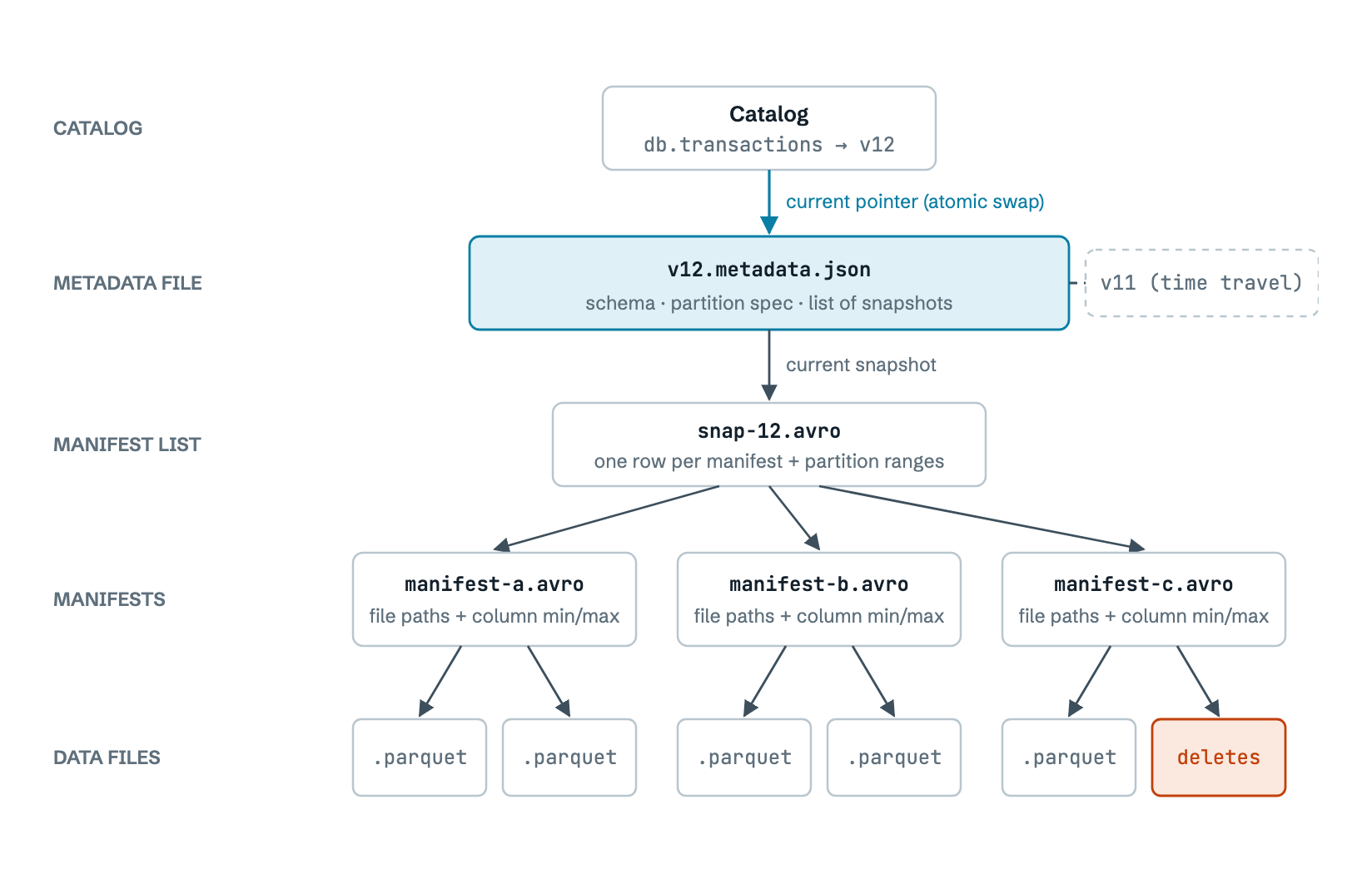
Figure 1. Every Iceberg table is a tree. The catalog holds one pointer. Everything below it is an immutable file on S3, so a reader always sees one consistent snapshot.

• A commit writes new data files, then new metadata, then swaps the catalog pointer in one atomic step. Readers see all of the change or none of it.
• A snapshot is an immutable list of files. Old snapshots stay until you expire them, which is what gives you time travel and rollback.
• Engines never list S3 folders. They read the manifests, which already know every file's partition and per-column min/max values.

How a read finds its data

That last point is where the speed comes from. Before opening a single Parquet file, the engine uses metadata to throw away files that can't contain a match. It skips data in three layers:

1. Partition pruning. Manifests record each file's partition values. With a table partitioned by account_id, months(transaction_date), a filter on those columns drops whole accounts and months before any file is opened.
2. File-level min/max statistics. Manifests also store each column's min and max for every file. A filter like source_ref = 'TX-88213' skips every file whose range can't contain that value.
3. Parquet row-group statistics. Inside each file that survives, rows are stored in chunks called row groups, each with its own min/max per column. Whole chunks are skipped the same way.

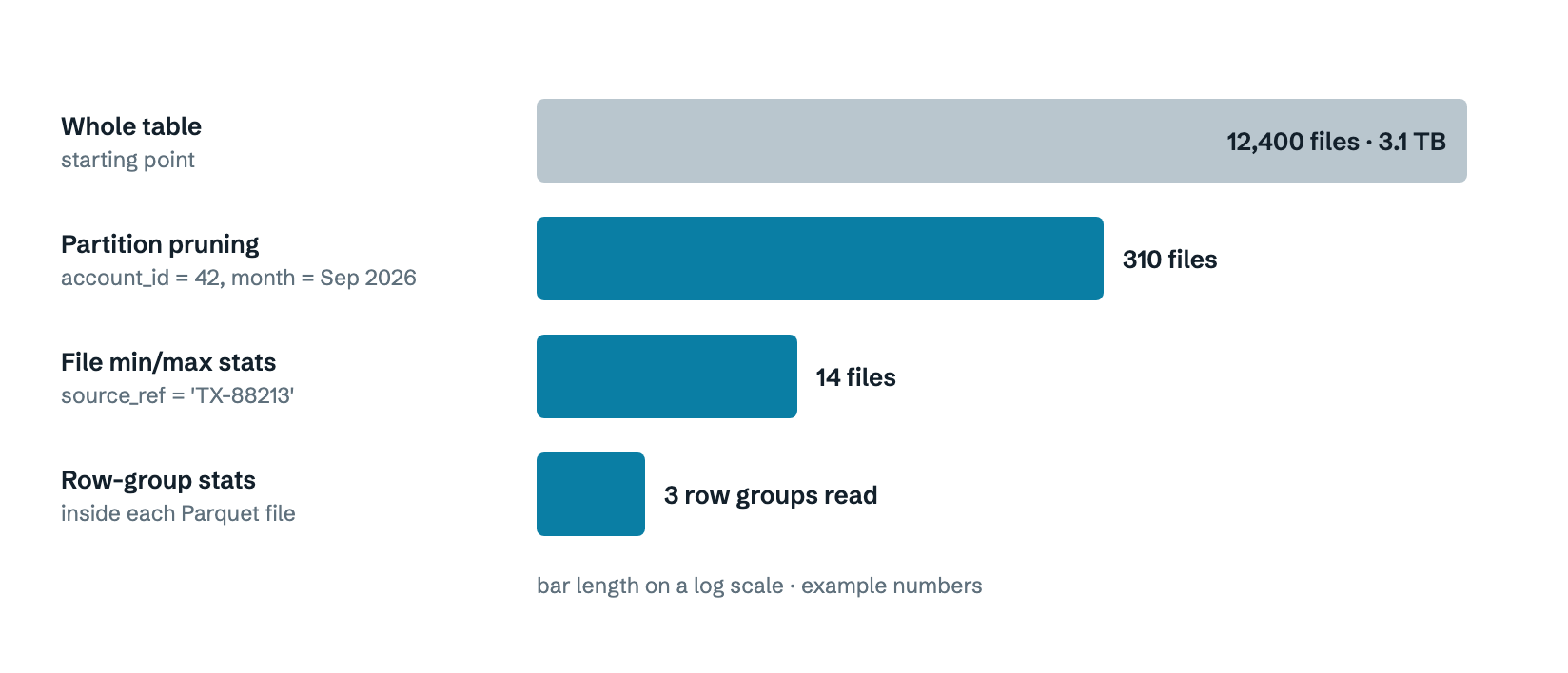
Figure 2. Three layers of skipping. The first two use only Iceberg metadata, so they cost almost nothing. A query that skips all three layers reads the whole table.

Partition pruning, with a real query

Our table is partitioned by (client_id, account_id, months(transaction_date)). Every file belongs to exactly one partition, a tuple such as (42, 7, 2026-10) and Iceberg writes that tuple into the file's manifest entry. Take this query:

SELECT id, amount
FROM db.transactions
WHERE client_id = 42 AND account_id = 7
  AND transaction_date >= TIMESTAMP '2026-10-01'
  AND transaction_date <  TIMESTAMP '2026-10-13';

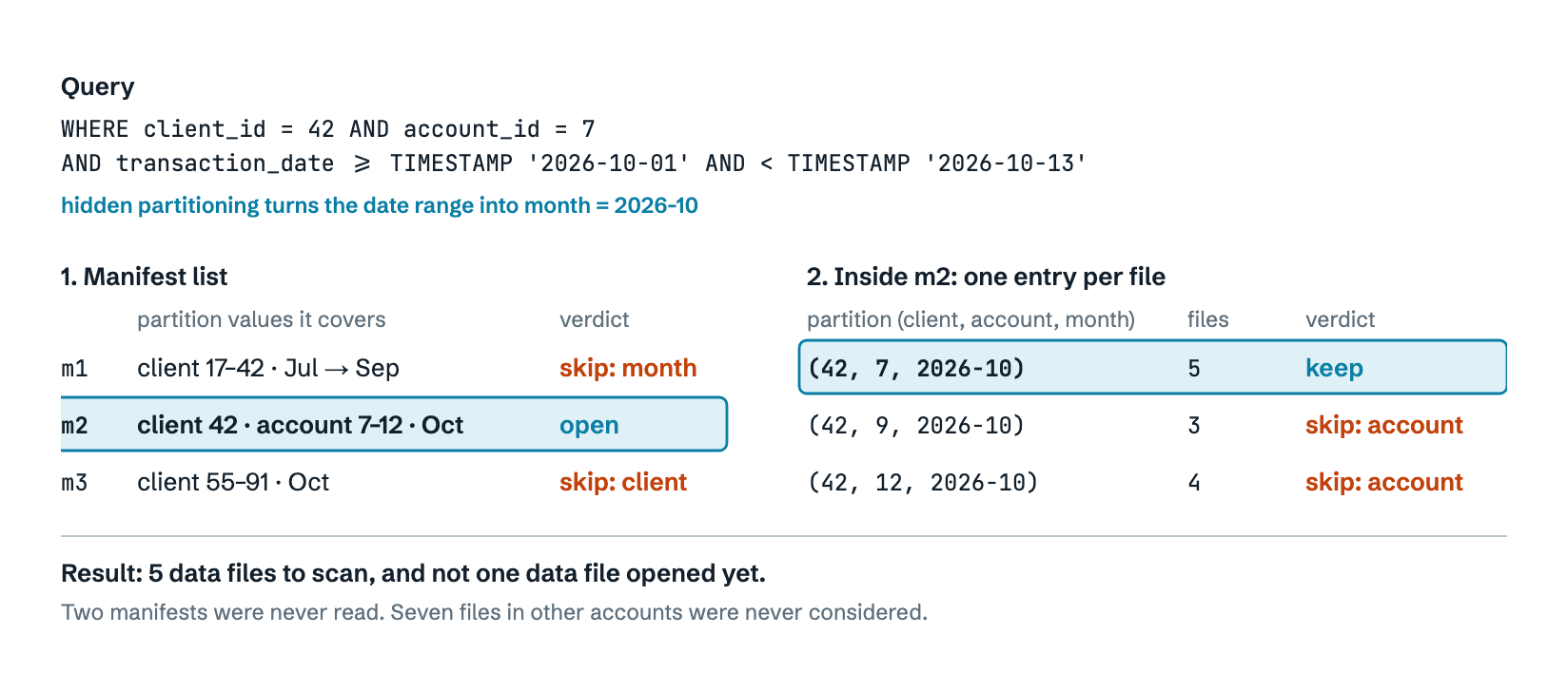
Figure 3. Partition pruning works in two passes over metadata. The manifest list rules out whole manifests and each remaining manifest rules out individual files. No data file is touched.

1. Translate the filter. The query never mentions a month. Because the partition spec says months(transaction_date), Iceberg derives month = 2026-10 from the date range on its own. This is hidden partitioning.
2. Read the manifest list. It stores, for each manifest, the lowest and highest value of every partition field it covers. m1 only covers July to September and m3 only covers clients 55 to 91, so neither is opened.
3. Read the surviving manifest. Each entry in m2 names one data file and its exact partition tuple. Only the five files in (42, 7, 2026-10) match.
4. Hand the five files to the next layer. All of this came from a handful of small metadata files.

When it doesn't help: the filter isn't on a partition column (reporting_tag, id, a map key), or the partition column is hidden inside a function the planner can't see through. The MERGE case study (Figure 14) is that second trap at full price.

File-level min/max statistics, with a real manifest

Partition pruning stops at the partition. The five files left in (42, 7, 2026-10) all have the same partition tuple, so it can't tell them apart. The next layer can. Each manifest entry also stores, for every column, the file's min value, max value, null count and row count. The query now adds one more filter:

  AND amount > 100000

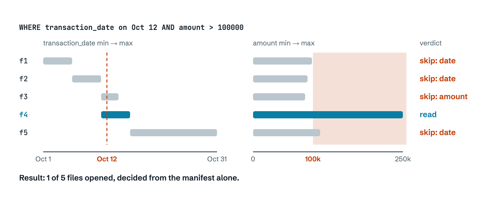
Figure 4. Each bar is one file's min → max range, read from its manifest entry. A file is opened only if every filter could match inside its ranges. Here only f4 passes both.

1. Check the date. f1 ends on Oct 6, f2 ends on Oct 11 and f5 starts on Oct 16, so none can hold Oct 12. f3 and f4 both span Oct 12 because they came from different write batches and nothing stops two files' ranges from overlapping.
2. Check the amount. f3's largest amount is 87,000, so amount > 100000 can't match. f4's maximum is 250,000, so it might.
3. Open f4 only. Inside it, the row-group statistics in the next section narrow things further.

When it doesn't help:

• Values are spread across every file. Unsorted data gives every file a range of Oct 1 → Oct 31, so all five are opened. That's why the sort order matters.
• The value is inside a map. All keys share one value column, so its min/max mixes every key together (Figure 21).
• The column has no statistics. By default Iceberg only collects them for the first 100 columns (write.metadata.metrics.max-inferred-column-defaults). For strings it keeps only the first 16 characters, which can blur long prefixes such as TXN-2026-10-….
• The filter is a not-equals. is_reversal != true can't be ruled out from a min/max range, but is_reversal = false can.

Row-group statistics, with a real file

The third layer happens inside a Parquet file, so it helps to see one. Parquet doesn't store a file as one block of rows. It cuts the rows into row groups, about 128 MB each by default (write.parquet.row-group-size-bytes). Inside each row group, every column is stored separately as a column chunk. At the end of the file sits a small footer that records, for every row group and every column, the min value, the max value and the null count.

Take a 512 MB file of October transactions, sorted by transaction_date and this query:

SELECT id, amount
FROM db.transactions
WHERE transaction_date = DATE '2026-10-12';

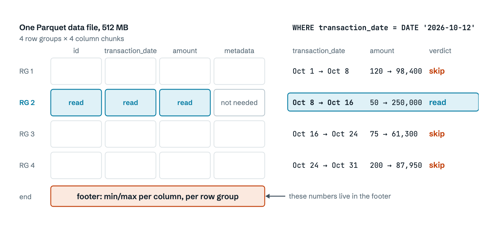
Figure 3. Left: how the file is laid out. Right: what its footer says. Only the highlighted chunks are fetched from S3: 3 of the 16 chunks.

Here is what the reader does, in order:

1. Reads the footer first. It's a few KB at the end of the file, fetched with one small S3 range request.
2. Checks the filter against each row group's range. Oct 12 can't be in Oct 1 → Oct 8, so row group 1 is skipped. Row group 2 covers Oct 8 → Oct 16, so it might contain matches. Row groups 3 and 4 start after Oct 12, so they're skipped.
3. Fetches only the column chunks it needs from row group 2: transaction_date to filter, plus id and amount to return. The metadata chunk is never downloaded. This is the columnar part of Parquet.
4. Filters the rows in memory. "Might contain" isn't "does contain". The reader still checks each row in row group 2 and keeps the ones dated Oct 12.

The amount column shows why the order matters. A filter like amount > 300000 skips all four row groups, because every max is below it. But amount = 5000 falls inside every range, so nothing can be skipped. Statistics only help on columns whose values are clustered and in our tables that means the column the data is sorted by. Shuffle the same rows randomly and every row group reports Oct 1 → Oct 31, so the Oct 12 query reads all four (Figure 18 shows that case).

	Layer 2: file statistics	Layer 3: row-group statistics
Where they live	Iceberg manifests	The footer of each Parquet file
What gets skipped	Whole files, without opening them	Row groups inside a file that's already been opened
Cost to check	Nothing extra; read during planning	One small read per surviving file
Matters most when	A partition has many files	A partition is one or a few large files

Lesson: a query is fast when its WHERE clause hits partition columns and columns whose values are tightly grouped inside each file. Everything in the "faster queries" section below is about making that true.

How writes commit and why they collide

Iceberg uses optimistic concurrency. Each writer assumes it is alone, does its work, then tries to swap the pointer. If someone else committed first, it has to re-check and retry.

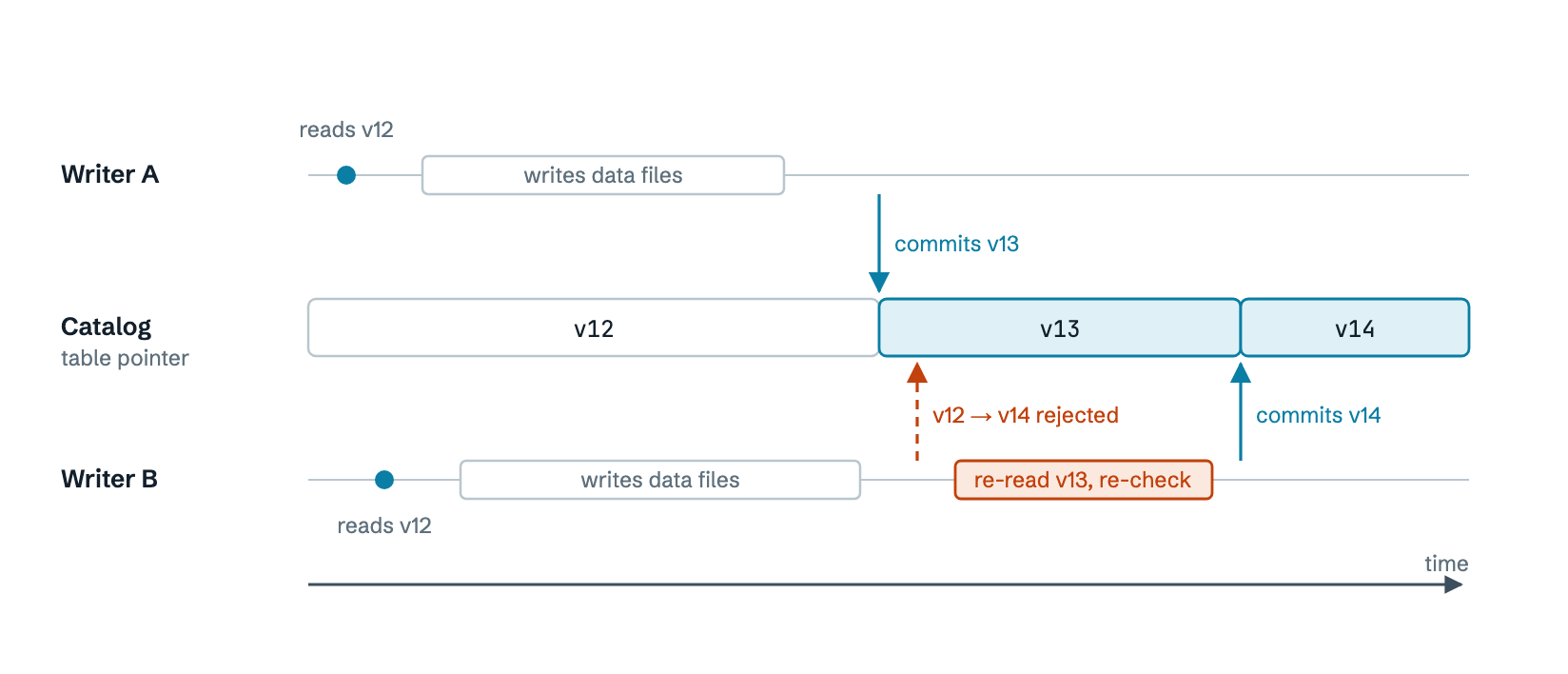
Figure 3. Conflicts are counted per table. Two jobs writing to different tables never wait on each other. Ten jobs writing to one table take turns.

Watch out: if you see many CommitFailedException retries, you have too many writers on one table. Batch small writes into fewer commits, keep independent write paths in separate tables and raise commit.retry.num-retries only as a safety net.

Updates and deletes: two strategies

Parquet files can't be edited. So when you UPDATE, DELETE or MERGE, Iceberg either rewrites files or writes small "delete files" next to them.

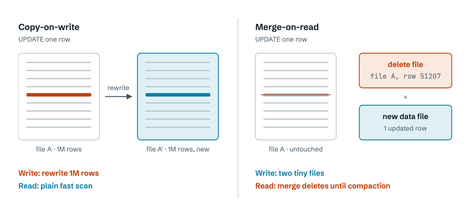
Figure 4. Copy-on-write makes writes pay. Merge-on-read makes reads pay and the bill grows with every unmerged delete file until compaction folds them back in.

Workload	Choose	Why
Frequent small MERGEs or updates (reconciliation, CDC)	Merge-on-read	Rewriting 512 MB to flip one flag is wasteful. Compact on a schedule.
Rare, large batch updates; read-heavy dashboards	Copy-on-write	Readers never pay a merge cost.
Append-only event logs	Either	No deletes, so the choice doesn't matter.

Set it per operation with write.update.mode, write.delete.mode and write.merge.mode.

Why does an update create a delete file?

Because Parquet files can't be edited, Iceberg has no real "update". Every UPDATE is carried out as two steps: delete the old version, then insert the new one. The write mode decides how the delete half is done.

Mode	Delete the old version	Insert the new version
Copy-on-write	Rewrite file A without the old row	The new row goes into that rewritten file
Merge-on-read	Write a delete file: "file A, row 51207 is gone"	Write a new data file holding the new row

So a delete file is merge-on-read's cheap way of saying "this old version no longer counts" without rewriting a 1M-row file. A plain DELETE works the same way minus the insert: it produces only a delete file. A MERGE is the same again: matched rows are deleted and re-inserted.

The three kinds of delete file

Kind	What it says	Who writes it	Cost at read time
Position delete	"file A, row 51207"	Spark, Athena and Trino UPDATE / DELETE / MERGE. The engine already scanned for the rows, so it knows exactly where they are.	Low: skip known positions
Equality delete	"any row where id = 42"	Streaming upserts (for example Flink), which don't look the row up first	High: every row of every older data file in scope is compared
Deletion vector (format v3)	A compact bitmap of deleted row positions, one per data file	The same engines, on v3 tables	Lowest: one small file per data file, replaced on each commit instead of piling up

Why the new row isn't deleted too

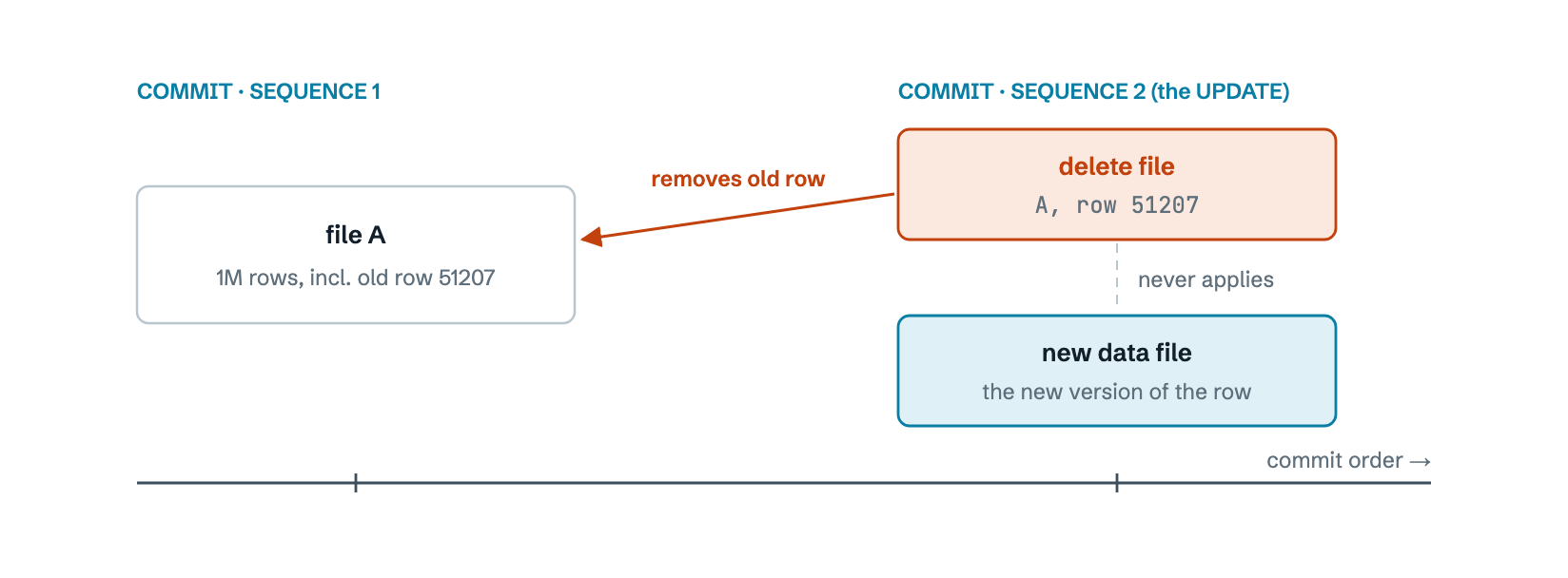
Figure 5. Every commit gets an increasing sequence number. A position delete names the exact file it applies to. An equality delete only applies to data files with a lower sequence number. Either way, the new row written in the same commit is safe.

The flow of a DELETE

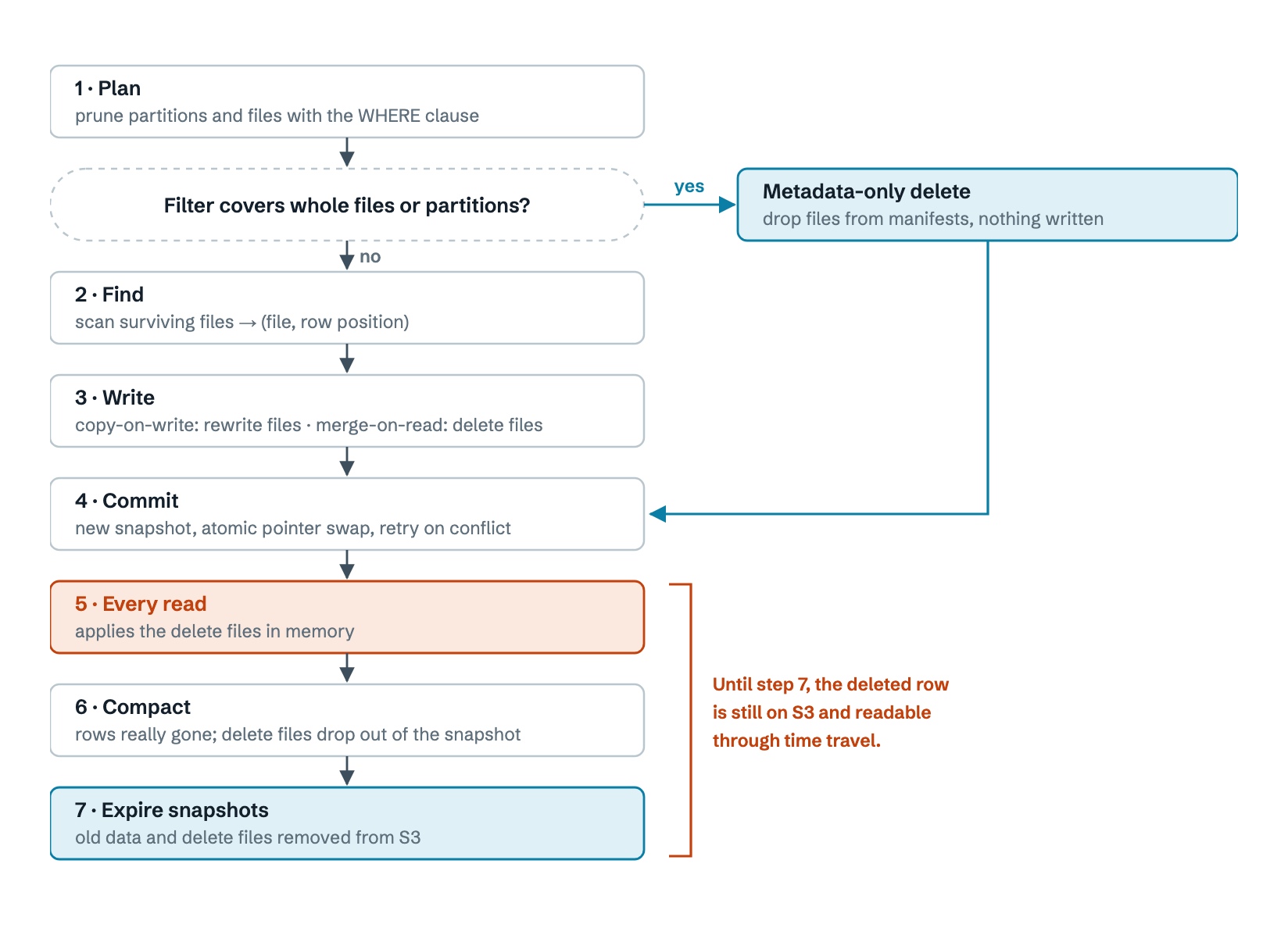
Figure 6. A DELETE from plan to physical removal. Figure 7 shows how an UPDATE differs.

The flow of an UPDATE

An update follows the same path as a delete, with two differences. It always writes the new row versions, so there is no metadata-only shortcut. And at step 3 the two write modes split: copy-on-write rewrites files, while merge-on-read writes a delete file plus a new data file. A MERGE works the same way: matched rows take this path and unmatched rows are plain inserts.

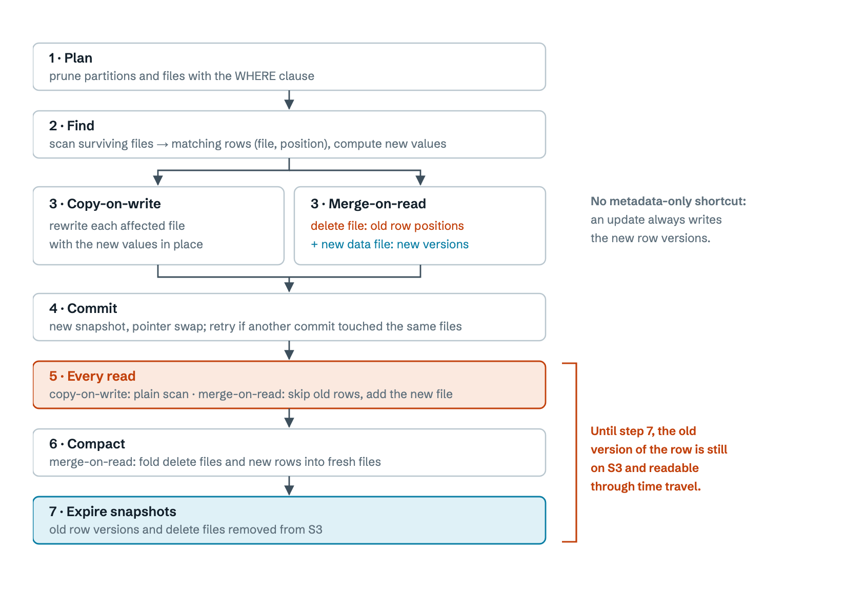
Figure 7. An UPDATE from plan to physical removal. The two write modes only differ at step 3; everything after that is shared, though compaction matters far more for merge-on-read.

Merge-on-read, step by step: what happens to the delete file?

A common misreading is that the one-row file gets merged into file A when you read it and the delete file then disappears. It doesn't. Reads never change anything on disk. The files are only combined when compaction runs and only removed from S3 when the old snapshot expires.

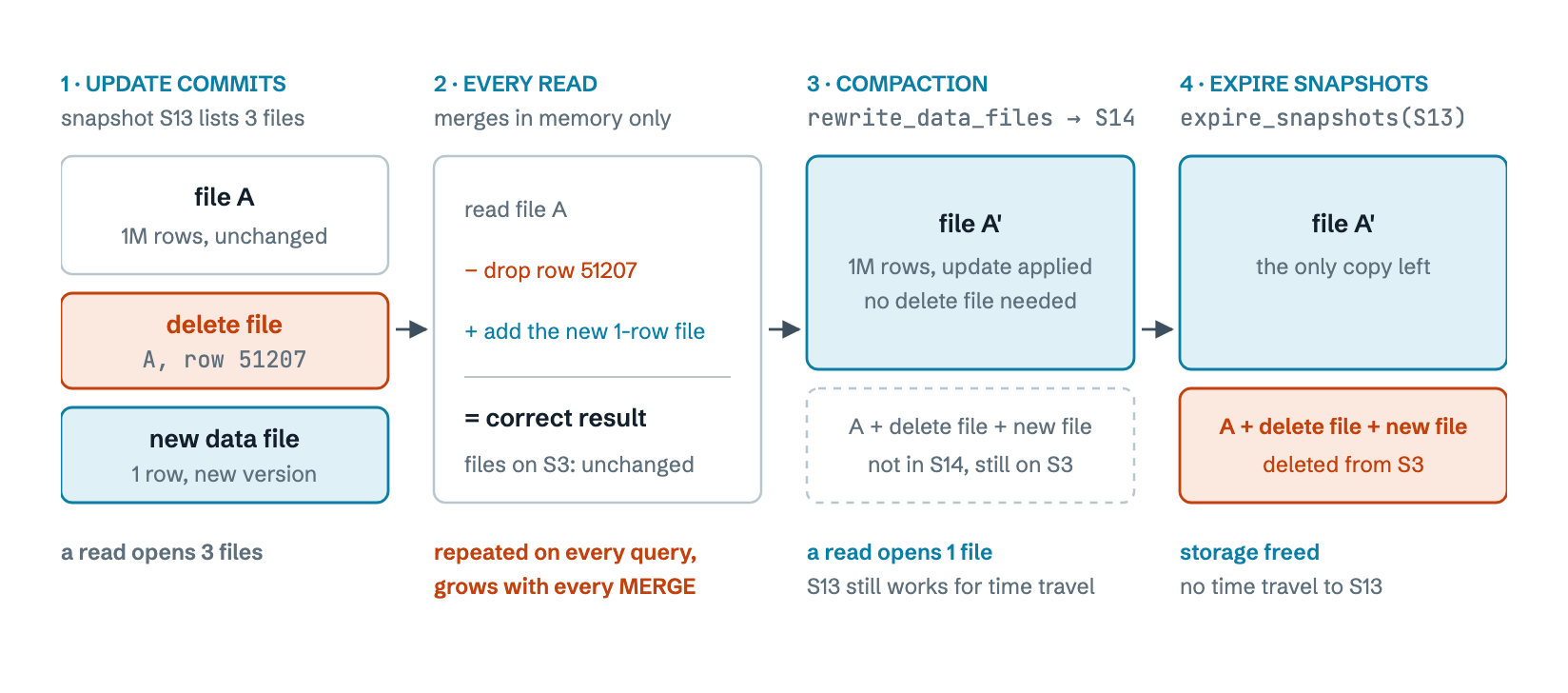
Figure 8. The lifecycle of one merge-on-read update. The delete file stops being used at step 3 and stops costing money at step 4.

• The one-row file is never appended to file A. Parquet files are immutable. Compaction writes a brand-new file A′ containing A's surviving rows plus the updated row and it may pack other small files from the same partition in with them.
• The delete file is dropped from the table, then from S3. Once every data file it points at has been rewritten, the new snapshot no longer lists it. It is physically deleted only when expire_snapshots removes the last snapshot that uses it.
• Until compaction runs, every read pays. Ten MERGEs on one partition mean ten delete files to apply on every query. That's why merge-on-read tables need compaction on a schedule.
• Newer format, same idea. Iceberg format v3 replaces per-commit position delete files with one compact "deletion vector" per data file. That makes reads cheaper, but you still need compaction and snapshot expiry.

Watch out: a deleted row stays on S3 until both compaction and snapshot expiry have run. If you handle data-removal requests (GDPR-style "erase my data"), your deadline includes those two jobs, not just the DELETE.

Tip: a delete whose filter lines up with partitions is almost free. On a table partitioned by account_id, months(transaction_date), DELETE ... WHERE account_id = 42 AND transaction_date < TIMESTAMP '2026-01-01' can drop whole files without writing anything.

When UPDATE and DELETE get slow

Almost every slow update or delete comes down to one of two things: step 2 has to scan too much, or step 3 has to write too much.

Situation	Why it's slow	What to do
The WHERE clause has no partition filter	Step 2 scans every file in the table to find the rows	Always include the partition columns, for example account and date range
Filtering on a map key, JSON field or a function of a column	No file can be skipped, so the scan is as wide as the partition filter allows	Promote the field to a real column; compare raw columns to literals
Scattered changes on a copy-on-write table	One changed row per file still rewrites the whole file. 1,000 rows spread over 1,000 files means 1,000 × 512 MB rewritten	Use merge-on-read for scattered changes, or sort the table so rows that change together live in the same files
Many small statements, such as an update per row in a loop	Each statement scans, writes, commits and adds a snapshot and its own delete files	Collect the changes and apply them in one MERGE (below)
Several jobs changing the same partitions at once	Conflicts are detected at commit time, after all the work is done, so the loser redoes the whole statement	One writer per table or partition at a time; batch changes; keep filters narrow so conflict checks are scoped
Delete files have piled up	Step 2 has to apply all existing delete files while it scans, before it can even find the rows	Compact merge-on-read tables on a schedule
Rewriting most of a partition with merge-on-read	You get a delete file listing almost every row, plus a full copy of the new rows. Reads pay for both until compaction	For bulk changes, use copy-on-write for that operation, or INSERT OVERWRITE the affected partitions
Equality deletes from streaming upserts	Every read compares rows against them	Compact often; prefer writers that produce position deletes

How MERGE works

MERGE takes a source of changes (a staging table or query) and applies it to a target table in one statement. It joins the two, decides per row whether to update, delete or insert, writes the results once and commits once.

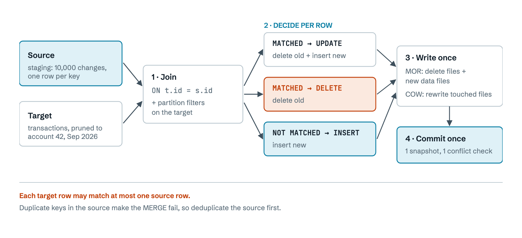
Figure 9. A MERGE is an update, a delete and an insert in one statement. However many rows it changes, it scans the target once and produces one snapshot.

Is MERGE the better way to change lots of rows?

For a batch of row-specific changes, yes. If you have 10,000 transactions that each need a different new value, a MERGE from a staging table does all of them in one pass. The same changes as 10,000 UPDATE statements repeat the whole flow 10,000 times.

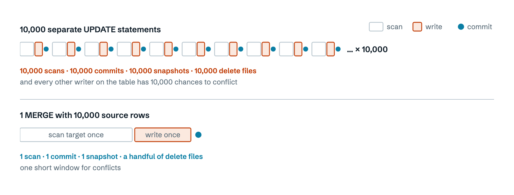
Figure 10. The win comes from batching, not from the keyword. Each statement carries a fixed cost: scan, commit, snapshot and conflict check. MERGE pays it once.

It isn't automatically better in every case:

• One set-based change: UPDATE t SET status = 'closed' WHERE batch_id = 7 is already a single pass. A MERGE would do the same work.
• Most of a partition changes: INSERT OVERWRITE of that partition is cheaper. It writes new files and drops the old ones, with no delete files at all.
• The target isn't pruned: a MERGE without partition filters on the target scans the whole table, which can be slower than a well-filtered UPDATE.

Writing a fast MERGE

MERGE INTO db.transactions t
USING (
  SELECT * FROM db.staging WHERE batch_id = 7      -- deduplicated: one row per id
) s
ON  t.id = s.id
AND t.account_id = 42                               -- prune the target
AND t.transaction_date >= TIMESTAMP '2026-09-01'
AND t.transaction_date <  TIMESTAMP '2026-10-01'
WHEN MATCHED AND s.op = 'delete' THEN DELETE
WHEN MATCHED AND t.status IS DISTINCT FROM s.status  -- skip rows that didn't change
  THEN UPDATE SET status = s.status, updated = s.updated
WHEN NOT MATCHED THEN INSERT *;                     -- Spark syntax; Athena needs a column list

• Put the target's partition filters in the ON clause. They prune the target scan and also narrow the conflict check, so concurrent jobs on other partitions don't clash.
• Deduplicate the source to one row per key. Duplicates make the MERGE fail.
• Skip no-op rows with a condition such as IS DISTINCT FROM. Without it, unchanged rows still get a delete and a re-insert.
• Keep the source small and filtered. A small source can be broadcast to every worker instead of shuffling both sides of the join.
• Run one MERGE per table per batch, not several in parallel on the same partitions.

Case study: the ON clause that scanned 130 GB

That first bullet cost us more than any other mistake. Our reconciliation rules are MERGE statements on the transactions table itself. The source query finds matched pairs and the MERGE flags them. The source was carefully filtered to one client, a few accounts and a 30-day window. The ON clause looked like this:

MERGE INTO db.transactions r
USING (
  SELECT client_id, array_agg(id) AS matched_ids
  FROM db.transactions
  WHERE client_id = 42 AND account_id IN (7)          -- source is pruned
    AND CAST(transaction_date AS DATE) >= date_parse('2026-09-01', '%Y-%m-%d')
    AND CAST(transaction_date AS DATE) <= date_parse('2026-09-30', '%Y-%m-%d')
  ...
) t
ON  r.client_id = t.client_id                         -- join condition, not a filter
AND contains(t.matched_ids, r.id)                     -- can't prune anything
WHEN MATCHED THEN UPDATE SET matched = true;

A MERGE is a join between the source and the target. Filters inside the USING subquery only prune the source's own scan and they don't carry over to the target. On the target side, nothing compared a partition column to a constant. r.client_id = t.client_id is a join condition and contains(array, r.id) is opaque to the planner. So Athena read every partition of the target to look for matches.

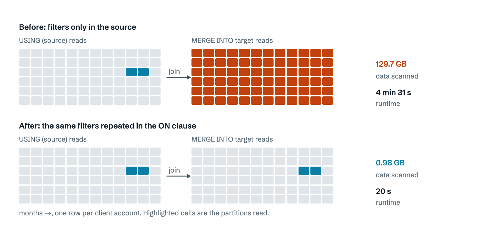
Figure 11. The same MERGE before and after. The source was always pruned. The target was not, until its filters were written into the ON clause.

The fix was to repeat the source's static filters on the target alias, inside ON:

ON  r.client_id = t.client_id
AND r.client_id = 42                                  -- static filters on the target:
AND r.account_id IN (7)                               -- these prune the target scan
AND CAST(r.transaction_date AS DATE) >= date_parse('2026-09-01', '%Y-%m-%d')
AND CAST(r.transaction_date AS DATE) <= date_parse('2026-09-30', '%Y-%m-%d')
AND contains(t.matched_ids, r.id)

One rule, one account, 30-day window	Before	After
Data scanned	129.72 GB	984 MB (99.2% less)
Runtime	4 min 31 s	20 s (about 13× faster)
Athena cost per run, at $5 per TB scanned	about $0.63	about $0.005

We then applied the same pattern to every rule file. Across the board, data scanned per query fell by about 98%, from over 100 GB to under 10 GB. Because a reconciliation run executes dozens of these rules one after another, the savings multiply.

The same pass also made some smaller fixes:

• Removed redundant date_trunc('month', CAST(transaction_date AS DATE)) filters. They added nothing the day-range filter didn't already say and a function wrapped around the column is the form planners are least likely to prune on.
• Trimmed unused columns from the UNNEST subqueries. Parquet is columnar, so every column you don't select is bytes never read and fewer bytes to shuffle into the join.
• Dropped an ORDER BY in the source. A MERGE doesn't care about the order of its source rows, so sorting them was pure cost.
• Wrote is_reversal = false instead of is_reversal != true. Both exclude NULL, but the equality form is a plain value that file statistics can check.

Lesson: every filter on the source of a MERGE belongs on the target too, written against the target alias in the ON clause. Then check the "Data scanned" figure in the query stats. In Athena, that number is also your bill.

Things to watch for

Most Iceberg problems are slow leaks. Each write leaves a little behind: a small file, a delete file, a snapshot, a manifest. Nothing breaks on day one. By month three queries are slow and the S3 bill has doubled.

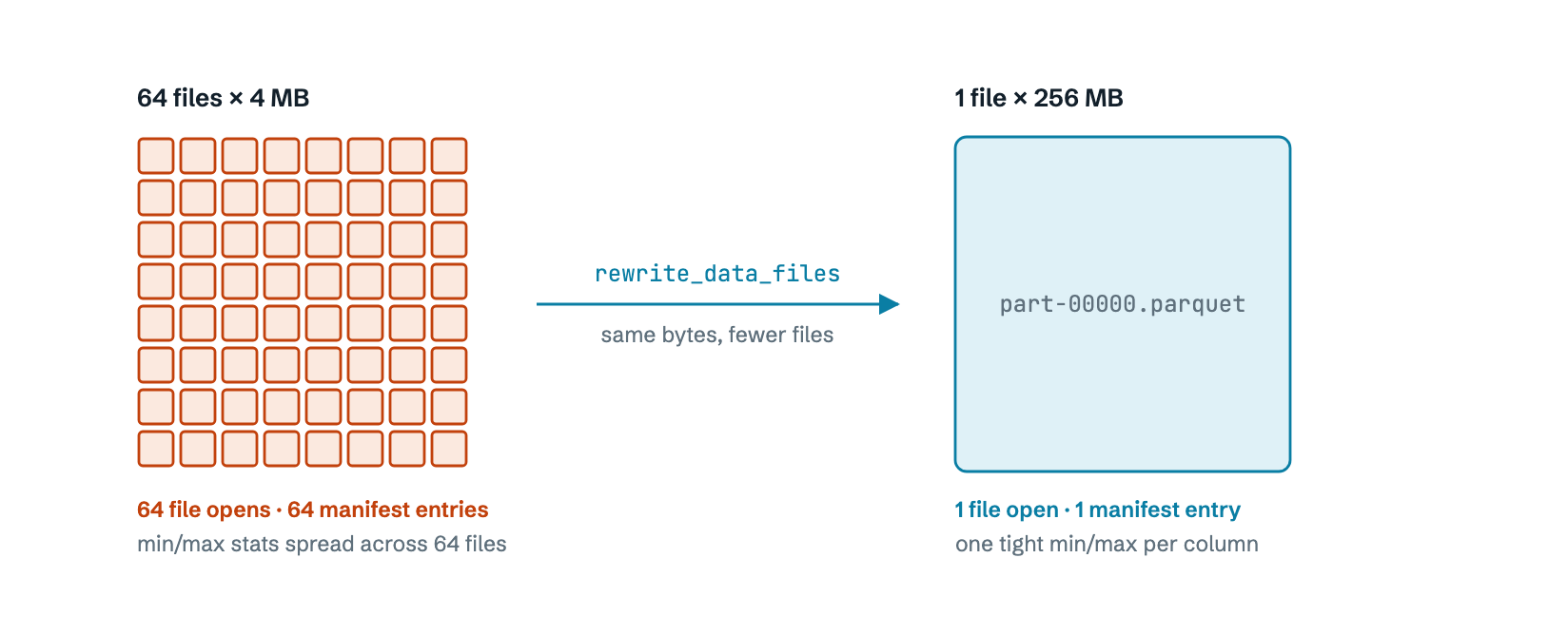
Figure 11. Small files are the most common Iceberg tax. Every file costs an S3 request, a manifest entry and some planning time, whatever its size.

Symptom	Usual cause	Fix
Queries slow down week by week	Thousands of small files from frequent small writes	Compact with rewrite_data_files; batch writes; set write.target-file-size-bytes
Reads slow after many MERGEs	Merge-on-read delete files piling up	Compact with a delete-file threshold; run rewrite_position_delete_files
Query planning takes seconds before any data is read	Too many snapshots or manifests	expire_snapshots, rewrite_manifests, cap write.metadata.previous-versions-max
S3 bill grows while the table doesn't	Unexpired snapshots; orphan files from failed jobs	expire_snapshots, then remove_orphan_files
A filter scans the whole partition anyway	Filtering on a value inside a map or JSON column, or on a function of a column	Promote the field to a real column; compare raw columns to literals
Millions of tiny partitions	Partitioning on a high-cardinality column (user, day for a quiet table)	Use coarser transforms like months(ts) or bucket(16, id)
Commit retries and timeouts under load	Many concurrent writers on one table	Fewer, larger commits; separate tables for separate write paths

Faster queries

1. Partition by how you filter and keep partitions big

Partition on the two or three columns almost every query filters on. Aim for each partition to hold at least a few hundred MB. Iceberg's hidden partitioning means you declare a transform once and users never see it:

CREATE TABLE db.transactions (...)
USING iceberg
PARTITIONED BY (client_id, account_id, months(transaction_date));

-- Users filter on the real column; Iceberg maps it to the month partition.
SELECT * FROM db.transactions
WHERE account_id = 42
  AND transaction_date >= TIMESTAMP '2026-09-01'
  AND transaction_date <  TIMESTAMP '2026-10-01';

Got it wrong? Partition specs can evolve without rewriting old data: ALTER TABLE db.transactions ADD PARTITION FIELD bucket(16, merchant_id).

2. Sort inside partitions so min/max statistics mean something

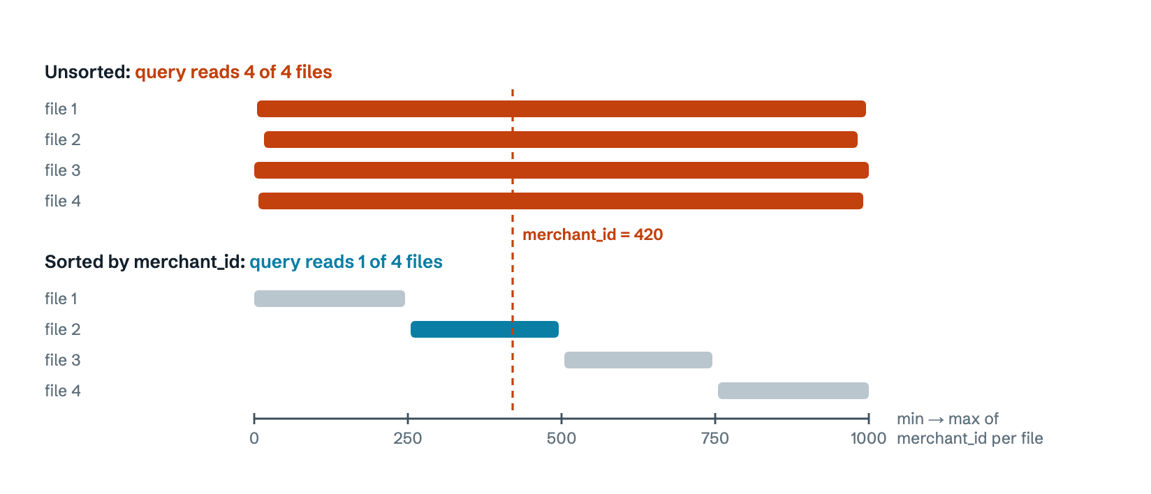
Figure 12. Each bar is one file's min-to-max range for merchant_id. Iceberg can only skip a file when the value you want falls outside its range, so random order makes the statistics useless.

ALTER TABLE db.transactions WRITE ORDERED BY merchant_id, source_reference;
-- Compaction then re-sorts existing data:
CALL catalog.system.rewrite_data_files(table => 'db.transactions', strategy => 'sort');

A worked example: our four-column sort order

Our transactions table is partitioned by (client_id, account_id, months(transaction_date)) and declares this sort order:

ALTER TABLE db.transactions
WRITE ORDERED BY transaction_date, client_id, account_id, reporting_tag;

It reads like clustering on four columns. In practice it clusters on one. Partitioning happens before sorting and every data file belongs to exactly one partition. So inside any file, client_id and account_id never change and sorting by a constant does nothing. transaction_date is a timestamp and almost unique, so reporting_tag only orders rows that share the exact same timestamp.

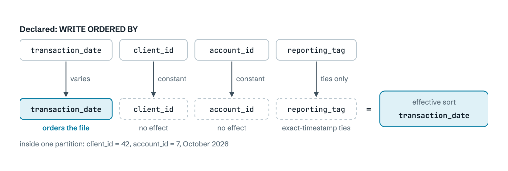
Figure 13. What the sort order does once partitioning has run. Only transaction_date changes the order of rows inside a file.

Rule of thumb: a sort column only helps if it still varies inside a partition and if the columns before it repeat often enough to leave ties for it to break.

To see what this means for queries, take one partition (one client, one account, October) holding six files and two filters our reconciliation rules use all the time:

• Query A, one day, every tag: transaction_date >= TIMESTAMP '2026-10-12' AND transaction_date < TIMESTAMP '2026-10-13'
• Query B, one tag, the whole month: reporting_tag = 'chargebacks'

Each rectangle below is one file's min/max box: its date range across, its tag range down. Iceberg reads a file only if the query's line or band touches its box.

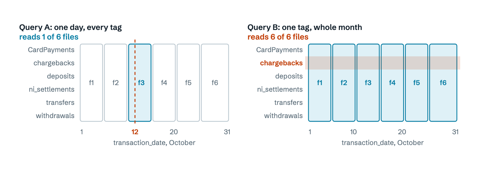
Figure 14. Rows written in sort order. Files become date stripes, so date filters skip well. Every stripe spans the alphabet of tags, from CardPayments to withdrawals, so a tag filter skips nothing.

Then compaction changes the picture. Our nightly job rewrites the last three months with strategy => 'sort', sort_order => 'zorder(transaction_date, client_id, account_id, reporting_tag)'. A sort_order passed to rewrite_data_files overrides the table's own order for the files it writes. Z-order interleaves the bits of each column, so each file ends up covering a block of dates and a block of tags. The constant partition columns drop out again, which leaves date and tag sharing the ordering.

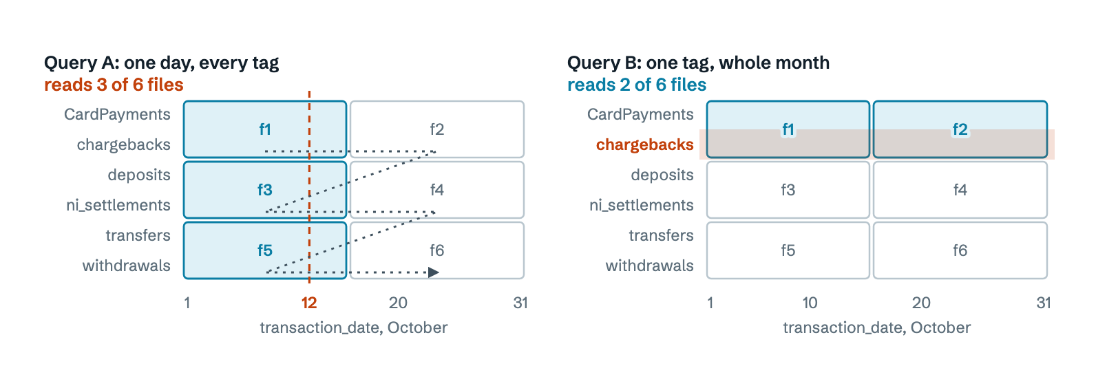
Figure 15. The same partition after z-order compaction. The dotted line is the order the curve visits the blocks. Date skipping gets weaker and tag skipping starts to work.

Filter	Linear by date	Z-order (date, tag)
A: one day, every tag	1 of 6 files	3 of 6
B: one tag, whole month	6 of 6	2 of 6
A and B together	1 of 6	1 of 6
client_id + account_id + month only	Partition pruning does all the work. Sort order doesn't matter.

There is one more layer. With a 512 MB target file size, a single account's month often fits in one to three files, so file-level skipping has little to choose from. The sort still pays off inside the file. Parquet stores min/max per row group and sorted rows give each row group a narrow date range.

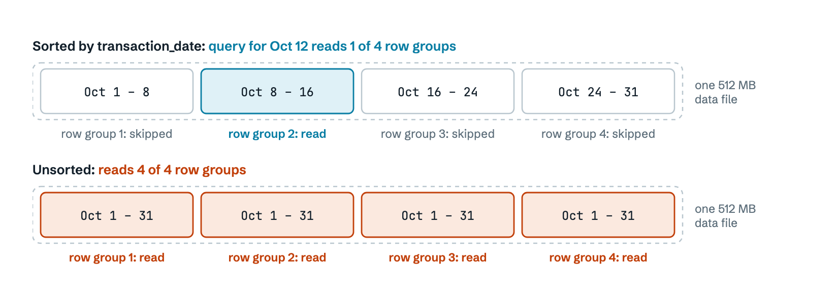
Figure 16. Inside one file. Even when a partition is a single file, sorting by date lets the reader skip most of it. Unsorted, it reads everything.

What we took from this:

• Partition columns in the sort order do nothing. Listing client_id and account_id is harmless, but it suggests clustering that isn't happening.
• A column behind a timestamp in a linear sort does nothing. If tag filters matter, either z-order on date and tag, or put the low-cardinality column first: WRITE ORDERED BY reporting_tag, transaction_date gives each tag its own date-sorted run. The cost is that a one-day, every-tag query then touches one run per tag.
• Don't let two layouts drift apart. New data lands linear by date. Compaction later turns it into z-order. Choose one layout on purpose, based on which filter your queries use most and set it in both places.
• The sort only helps filters on the raw column. CAST(transaction_date AS DATE) or DATE_FORMAT(...) can hide the range from the planner (see tip 5 below).
• Check the layout, don't guess it. In Spark, the files metadata table shows each file's ranges:

SELECT file_path, record_count,
       readable_metrics.transaction_date.lower_bound AS date_min,
       readable_metrics.transaction_date.upper_bound AS date_max,
       readable_metrics.reporting_tag.lower_bound    AS tag_min,
       readable_metrics.reporting_tag.upper_bound    AS tag_max
FROM catalog.db.transactions.files
WHERE partition.client_id = 42 AND partition.account_id = 7
ORDER BY date_min;
-- Narrow, non-overlapping date ranges: date skipping works.
-- tag_min = 'CardPayments' and tag_max = 'withdrawals' on every file: tag skipping doesn't.

3. Don't hide hot fields inside maps or JSON

A MAP<STRING,STRING> column is handy for odd extra fields. But Parquet stores every map key in one column and every value in another, so the min/max statistics mix all keys together.

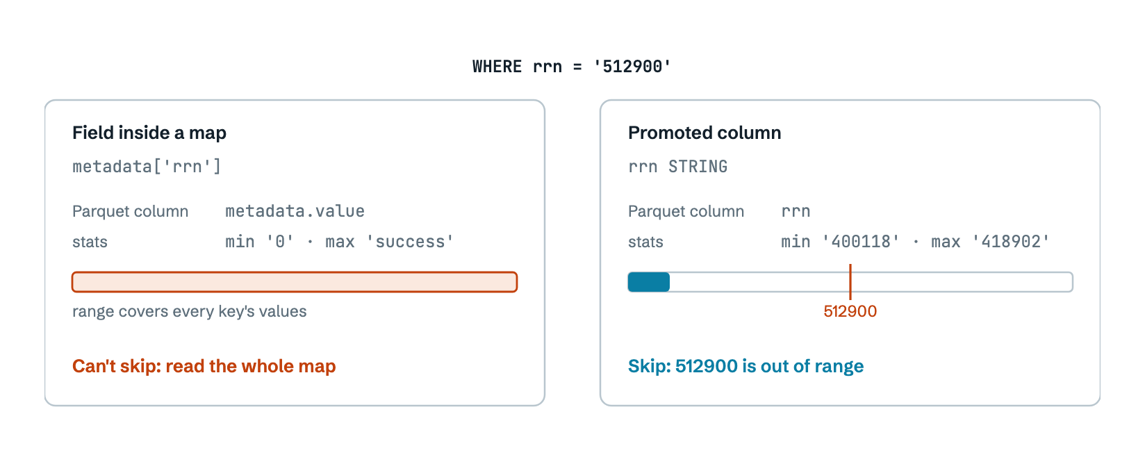
Figure 17. Same data, two layouts. The map version must read and rebuild the whole map for every row. The promoted column lets Iceberg skip the file from metadata alone.

How a map column behaves in each of the three skipping layers:

• Partition pruning still works, as long as the query also filters on partition columns. That is the only layer left.
• File min/max is useless. The "metadata values" range covers rrn, status, amount and every other key mixed together, so no file can ever be ruled out.
• Row-group statistics are useless too, for the same reason. Engines like Athena (Trino) and Spark don't push a map lookup into the scan at all. They read the column, rebuild the map for each row, then filter.

	Top-level typed column	Key inside a map
Files skipped by min/max	Yes	No
Bytes read	Only that column	The entire map, all keys and values, for every row in the scanned partitions
CPU	Compare values directly	Rebuild the map per row, look up the key, often CAST the string
As a join key	The engine can use the other side's values to skip files on this side (dynamic filtering)	Can't. ON element_at(l.metadata, 'rrn') = r.x is an expression, so every row is evaluated

A map is often one of the widest columns in the table, so reading all of it to check one key can be most of a query's scan.

What to do about it:

1. Promote the keys you filter or join on to top-level columns. In Iceberg, ALTER TABLE ... ADD COLUMNS only changes metadata, so it's cheap. Fill the new column at ingestion, backfill old rows once with an UPDATE or MERGE and keep the map for rare keys.
2. Give them real types, for example amounts as decimal(32,4), so min/max statistics and comparisons are correct.
3. Add Bloom filters for exact lookups on high-cardinality columns like IDs: 'write.parquet.bloom-filter-enabled.column.rrn'='true'. Check that your engine version actually reads them.
4. Rewrite the queries to use the new columns. Filters and join keys then get file skipping and dynamic filtering for free.

4. Joins: cheap when pruned, expensive when not

A join isn't slow by itself. On a data lake, its cost comes from three things:

• Bytes scanned on each side. If both tables are filtered on their partition columns, each side is already small before the join starts. Put the partition filters on every table in the join, not just one.
• The join key. On a plain column, Athena and Trino build a filter from the smaller side's keys and use it to skip files on the bigger side. A map lookup, CAST or function in the ON clause turns that off.
• Rows exploded before the join. UNNEST and CROSS JOIN UNNEST(...) on arrays multiply rows before the join and can cost more than the join itself. Filter first, unnest last.

So joins on well-pruned plain columns are fine. A join keyed on map values over a wide date range is where queries get slow and it's slow for the map reasons above, not because it's a join.

5. Compare raw columns to literals

transaction_date >= TIMESTAMP '2026-09-01' prunes reliably. Wrapping the column in a function or cast, as in CAST(transaction_date AS date) = ..., may not, depending on the engine. Put the transformation on the literal side.

Cheaper, leaner storage

Iceberg never deletes anything by itself. Every rewrite leaves the old files in place for old snapshots. You need a maintenance routine and the order matters.

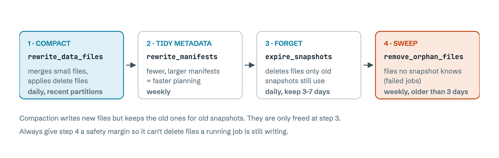
Figure 18. Compaction alone makes queries faster but storage bigger. Storage only shrinks once expired snapshots release the old files.

-- Spark (Iceberg procedures)
CALL catalog.system.rewrite_data_files(table => 'db.transactions',
  where => 'transaction_date >= current_date() - INTERVAL 7 DAYS');
CALL catalog.system.rewrite_manifests('db.transactions');
CALL catalog.system.expire_snapshots(table => 'db.transactions',
  older_than => TIMESTAMP '2026-10-22 00:00:00', retain_last => 10);
CALL catalog.system.remove_orphan_files(table => 'db.transactions');

-- Athena equivalents
OPTIMIZE db.transactions REWRITE DATA USING BIN_PACK;
VACUUM db.transactions;

Settings that shrink the bill

Setting	Suggested value	Effect
write.parquet.compression-codec	zstd	Usually smaller files than snappy for similar read speed. It's the default in recent Iceberg versions.
write.target-file-size-bytes	128–512 MB	Fewer files, fewer S3 requests
write.metadata.delete-after-commit.enabled	true	Old metadata.json files are cleaned up automatically
write.metadata.previous-versions-max	10–50	Caps how many old metadata files are kept
write.metadata.metrics.default	truncate(16), with none for wide text columns you never filter on	Smaller manifests on wide tables
Column types	decimal, date, bigint instead of string	Better compression and min/max that compares correctly

What map columns cost in storage

• Key names are stored on every row. The strings "rrn", "status" and so on repeat for each row. Parquet's dictionary encoding and compression shrink them well because they repeat, so this overhead is real but modest.
• Values compress worse than typed columns. Everything is a STRING, so an amount is stored as text instead of a decimal. Mixing many keys in one column also makes a messier dictionary than separate columns would.
• The bigger cost is reading, not storing. Athena bills per byte scanned and every filter on a map key scans the whole map.

Simpler queries, easier changes

Performance tuning is wasted if nobody can safely change the queries afterwards. These habits kept our SQL short and our migrations boring.

Typed columns beat map lookups in readability too

Before

SELECT *
FROM transactions t
WHERE CAST(element_at(t.metadata,
        'ReconAmount') AS decimal(32,4)) > 1000
  AND COALESCE(t.metadata['rrn'],
        t.metadata['reference']) = ?

After

SELECT *
FROM transactions t
WHERE t.recon_amount > 1000
  AND t.rrn = ?

The second version is shorter, prunes files and fails loudly at write time if the data is the wrong type, not silently at query time.

More habits

• Lean on hidden partitioning. Never ask users to add a separate month = '2026-09' filter. They filter on the timestamp; Iceberg does the rest.
• Evolve schemas freely, but never reuse a column name for new meaning. Iceberg tracks columns by ID, so add, rename and drop are safe metadata changes. Readers of old dashboards are not.
• One table per write path, views for reading. Separate tables keep writers from colliding (Figure 3). A UNION ALL view gives analysts one place to query and engines push filters down into it.
• Debug with time travel. SELECT ... FOR VERSION AS OF 4129... shows the table before a bad job. `CALL catalog.system.rollback_to_snapshot(..