Learn Trapping Rain Water, Top K Frequent and Selection Sort with Step-by-Step Visualization 👀👀

Question

Hoi hoi!

I’m @nyaomaru, a frontend engineer who has been obsessed with ramen lately. 😸🍜

Have you used DSA View View already? 👀👀

https://dev.to/nyaomaru/i-built-a-tool-to-visualize-dsa-letearn-together-dsa-view-view--djo

DSA View View allows you to understand DSA by visualizing how your implementation actually runs.

In the previous articles, we looked at problems like:

• Two Sum
• Binary Search
• Bubble Sort
• Valid Parentheses
• Reverse Linked List
• Maximum Depth of Binary Tree
• Number of Islands
• Invert Binary Tree
• Course Schedule

https://dev.to/nyaomaru/is-learning-dsa-boring-lets-use-dsaew-view-two-sum-binary-search-and-bubble-sort-374o

https://dev.to/nyaomaru/learn-valid-parentheses-reverse-lin-list-and-tree-max-depth-with-step-by-step-visualization-in-3o09

https://dev.to/nyaomaru/learn-number-of-islands-invert-binatree-and-course-schedule-with-step-by-step-visualization-in-5947

This time, let's try three more problems:

• Trapping Rain Water
• Top K Frequent Elements
• Selection Sort

These three problems introduce some very useful ways of thinking

Shrink a problem from both sides
Count first, then organize by frequency
Repeatedly select the next value

Once again, the implementations are not necessarily huge.

But there are several changing values that we need to keep in our heads.

So instead of only reading the final code,

Let's view what actually happens. 👀👀

---

🌧️ Trapping Rain Water

Let's start with Trapping Rain Water.

Suppose we have these heights

[0, 1, 0, 2, 1, 0, 1, 3]

If we draw them as walls, it looks roughly like this.

              █
      █       █
  █   █ █   █ █
-----------------
0 1 0 2 1 0 1 3

Rain falls from above.

Some water escapes.

But some water becomes trapped between taller walls.

For example

      █~~~~~~~█
  █~~~█~~~~~~~█
-----------------

So the question is

How much water can be trapped?

At first, I found this problem quite confusing. 😿

Because the amount of water above one position depends on walls somewhere else.

So what information do we actually need?

How Much Water Fits Above One Position?

Imagine this position

left wall     right wall
    █             █
    █      x      █
    █      █      █

The water level cannot be higher than the shorter side.

So the maximum possible water level is

Math.min(leftMax, rightMax);

Then we subtract the current height.

Conceptually:

water = min(leftMax, rightMax) - currentHeight

That's the basic idea.

But do we really need to calculate both sides again for every position?

No.

We can use two pointers.

Two Pointers

Here is the implementation.

function trap(height: number[]): number {
  let left = 0;
  let right = height.length - 1;

  let leftMax = 0;
  let rightMax = 0;

  let water = 0;

  while (left <= right) {
    if (height[left] <= height[right]) {
      if (height[left] >= leftMax) {
        leftMax = height[left];
      } else {
        water += leftMax - height[left];
      }

      left++;
    } else {
      if (height[right] >= rightMax) {
        rightMax = height[right];
      } else {
        water += rightMax - height[right];
      }

      right--;
    }
  }

  return water;
}

There are several important values.

left
right
leftMax
rightMax
water

This is exactly the kind of code where I understand every variable individually,

but then lose track of all of them together. 😹

Let's follow a smaller example.

[2, 0, 1, 3]

Start From Both Ends

At first

left = 0
right = 3

[2, 0, 1, 3]
 ↑        ↑
left    right

The heights are:

height[left]  = 2
height[right] = 3

Since

2 <= 3

we process the left side.

There is a wall with height 2.

So

leftMax = 2

Then move left.

[2, 0, 1, 3]
    ↑     ↑
   left right

Now We Can Trap Water

The current height is

0

But we already know there is a wall of height 2 on the left.

And the right side is currently at least as high as that.

So this position can hold

leftMax - height[left]
= 2

Therefore

water = 2

Move again.

[2, 0, 1, 3]
       ↑  ↑
      left right

Now

height[left] = 1
leftMax = 2

So

2 - 1 = 1

One more unit of water.

water = 3

Eventually we reach the final wall.

Done! 🎉

Why Can We Process the Shorter Side?

This part is the important idea.

Suppose

height[left] <= height[right]

Then we already know there is a wall on the right that is at least as tall as the current left wall.

So for the current left position, the limiting factor is the best wall we have seen from the left.

That's why we can safely calculate

leftMax - height[left];

without knowing every future wall.

The same logic works from the other side.

If

height[right] < height[left]

we process the right side using rightMax.

So the algorithm keeps shrinking the unknown area

L → → →     ← ← ← R

until everything has been processed.

Complexity

Each pointer only moves across the array once.

Time:  O(n)
Space: O(1)

👀 Let's View View It

This problem is a perfect example of why I like visualization.

The code contains

left
right
leftMax
rightMax
water

And they all change at different times.

When I only read

water += leftMax - height[left];

I might ask:

• Why are we using leftMax here?
• What is rightMax right now?
• Why did we move left instead of right?
• How much water have we already counted?
• Which part of the array is still unprocessed?

😿

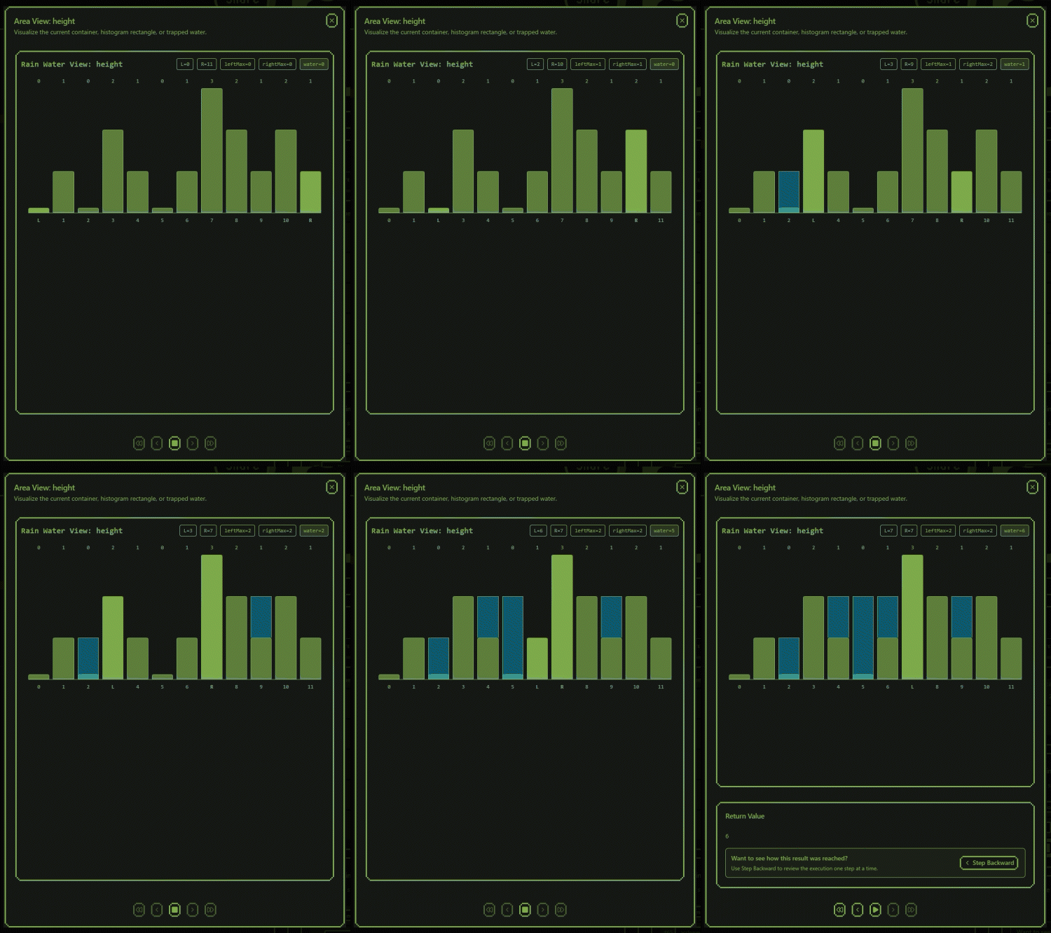
https://dsa-view-view.vercel.app/#s=j.eyJlIjoidHJhcHBpbmctcbi13YXRlciIsImwiOiJ0eXBlc2NyaXB0IiwibSI6InZlcmlmaWNhdGlvbiIsInYiOjF9

Step by step, we can actually watch the search area shrink.

L         R
↓         ↓
[2, 0, 1, 3]

    L     R
    ↓     ↓
[2, 0, 1, 3]

       L  R
       ↓  ↓
[2, 0, 1, 3]

And at the same time

leftMax
rightMax
water

keep changing.

The algorithm is really asking

Which side can I safely solve right now?

Then it solves that side and moves inward. 🌧️😸

---

🔢 Top K Frequent Elements

Next, let's find the Top K Frequent Elements.

Suppose we have

[1, 1, 1, 2, 2, 3]

and

k = 2

How often does each number appear?

1 → 3 times
2 → 2 times
3 → 1 time

So the two most frequent values are

[1, 2]

Simple enough.

But how should we implement it?

First, Count Everything

The first thing we need is frequency.

We can use a Map.

const frequency = new Map<number, number>();

Then count each value.

for (const num of nums) {
  frequency.set(num, (frequency.get(num) ?? 0) + 1);
}

For

[1, 1, 1, 2, 2, 3]

we get

frequency = {
  1 → 3
  2 → 2
  3 → 1
}

Nice.

But we still need the top K.

Of course, we could sort everything by frequency.

But there is another interesting approach.

Use Frequency as an Index

The maximum possible frequency is

nums.length

So we can create buckets.

const buckets: number[][] = Array.from({ length: nums.length + 1 }, () => []);

The index represents frequency.

For example

bucket[1] = values appearing 1 time
bucket[2] = values appearing 2 times
bucket[3] = values appearing 3 times

For our example:

frequency = {
  1 → 3
  2 → 2
  3 → 1
}

the buckets become

index 0 → []
index 1 → [3]
index 2 → [2]
index 3 → [1]

That's pretty interesting. 👀👀

Instead of asking

What is the frequency of this number?

we reverse the relationship

Which numbers have this frequency?

Implementation

Here is the full implementation:

function topKFrequent(nums: number[], k: number): number[] {
  const frequency = new Map<number, number>();

  for (const num of nums) {
    frequency.set(num, (frequency.get(num) ?? 0) + 1);
  }

  const buckets: number[][] = Array.from({ length: nums.length + 1 }, () => []);

  for (const [num, count] of frequency) {
    buckets[count].push(num);
  }

  const result: number[] = [];

  for (let count = buckets.length - 1; count >= 0; count--) {
    for (const num of buckets[count]) {
      result.push(num);

      if (result.length === k) {
        return result;
      }
    }
  }

  return result;
}

Let's follow it.

Step 1: Build the Frequency Map

Start

frequency = {}

Read the first 1. And another one and another...

1 → 1
1 → 2
1 → 3

Then 2. And another one.

1 → 3
2 → 1
2 → 2

Finally 3.

1 → 3
2 → 2
3 → 1

Done.

Step 2: Put Values Into Buckets

Now

buckets[count].push(num);

For

1 → 3

we do

buckets[3].push(1)

For

2 → 2

we do

buckets[2].push(2)

And

3 → 1

becomes

buckets[1].push(3)

So

0: []
1: [3]
2: [2]
3: [1]

Step 3: Read From Highest Frequency

We want the most frequent values.

So don't start at 0. Start from the end.

3 → [1]
2 → [2]
1 → [3]

Take 1.

result = [1]

We still need one more. Move down.

Take 2.

result = [1, 2]

Now

result.length === k

So return.

Done! 🎉

Why Is This Interesting?

I like this solution because the second structure changes our perspective.

The Map says

value → frequency

The buckets say

frequency → values

Same information. But different direction.

And suddenly finding the most frequent values becomes easy.

We just walk backward through the buckets.

Complexity

We count every number once.

We distribute every unique number into a bucket.

Then we walk through the buckets.

Time:  O(n)
Space: O(n)

👀 Let's View View It

There are two transformations happening here.

First

nums
 ↓
frequency Map

Then

frequency Map
 ↓
buckets

Then

buckets
 ↓
result

Reading the final implementation, it can be easy to miss why we're building two different data structures.

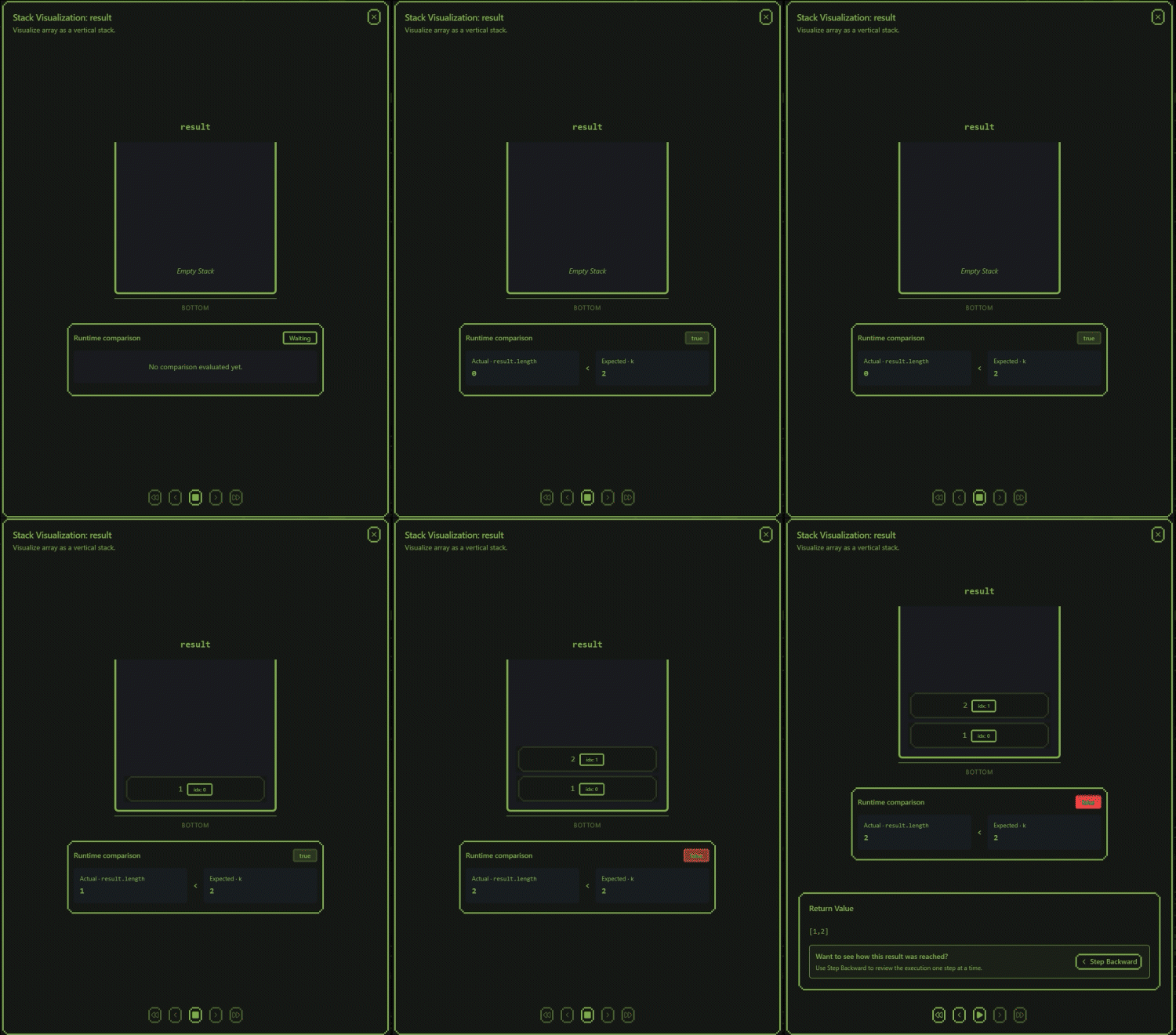
https://dsa-view-view.vercel.app/#s=j.eyJlIjoidG9wLWstZnJlcbnQiLCJsIjoidHlwZXNjcmlwdCIsIm0iOiJ2ZXJpZmljYXRpb24iLCJ2IjoxfQ

With the runtime visible, we can follow the data changing shape.

[1, 1, 1, 2, 2, 3]
        ↓ count
1 → 3
2 → 2
3 → 1
        ↓ bucket
1: [3]
2: [2]
3: [1]
        ↓ highest first
[1, 2]

That's the part I like.

We don't magically find the top K.

We reorganize the information until the answer becomes easy to read. 🔢😸

---

👉 Selection Sort

Finally, let's sort something again!

We already looked at Bubble Sort in a previous article.

This time, let's try Selection Sort.

Suppose we have

[5, 3, 4, 1, 2]

We want

[1, 2, 3, 4, 5]

Selection Sort follows a very simple idea

Find the smallest remaining value and move it to the front.

Then repeat.

First Pass

Start

[5, 3, 4, 1, 2]
 ↑
 i

Assume the first value is currently the smallest.

minIndex = 0

Then scan everything to the right.

5 vs 3

3 is smaller.

So:

minIndex = 1

Then:

3 vs 4

No change.

Then

3 vs 1

1 is smaller.

minIndex = 3

Finally

1 vs 2

Still 1.

So the smallest value is at index 3.

Swap

[5, 3, 4, 1, 2]
 ↑        ↑
 i       min

↓

[1, 3, 4, 5, 2]

Now the first position is finished.

[1 | 3, 4, 5, 2]
 ↑
sorted

Repeat

Next, start from index 1.

[1 | 3, 4, 5, 2]
     ↑
     i

Find the smallest value in

[3, 4, 5, 2]

That's 2.

Swap.

[1, 2 | 4, 5, 3]

Again.

Find the smallest remaining value.

3

Eventually

[1, 2, 3, 4, 5]

Sorted! 🎉

Implementation

function selectionSort(nums: number[]): number[] {
  for (let i = 0; i < nums.length - 1; i++) {
    let minIndex = i;

    for (let j = i + 1; j < nums.length; j++) {
      if (nums[j] < nums[minIndex]) {
        minIndex = j;
      }
    }

    if (minIndex !== i) {
      [nums[i], nums[minIndex]] = [nums[minIndex], nums[i]];
    }
  }

  return nums;
}

There are two important indexes.

i
minIndex

And also

j

which searches through the unsorted area.

Why Is It Called Selection Sort?

Because each pass selects the smallest remaining value.

Find smallest
  ↓
Select it
  ↓
Move it to the front
  ↓
Repeat

That's basically the whole algorithm.

Complexity

For every position, we search through the remaining values.

So

Time: O(n²)

We sort the array in place.

Space: O(1)

Selection Sort is not something I would normally choose for sorting a huge production dataset. 😹

But as a learning algorithm, it is wonderfully visual.

👀 Let's View View It

The implementation contains nested loops.

for (let i = 0; i < nums.length - 1; i++) {
  let minIndex = i;

  for (let j = i + 1; j < nums.length; j++) {

Reading it, I might lose track of:

• Which area is already sorted?
• Where is i?
• Where is j?
• What does minIndex currently point to?
• When exactly does the swap happen?

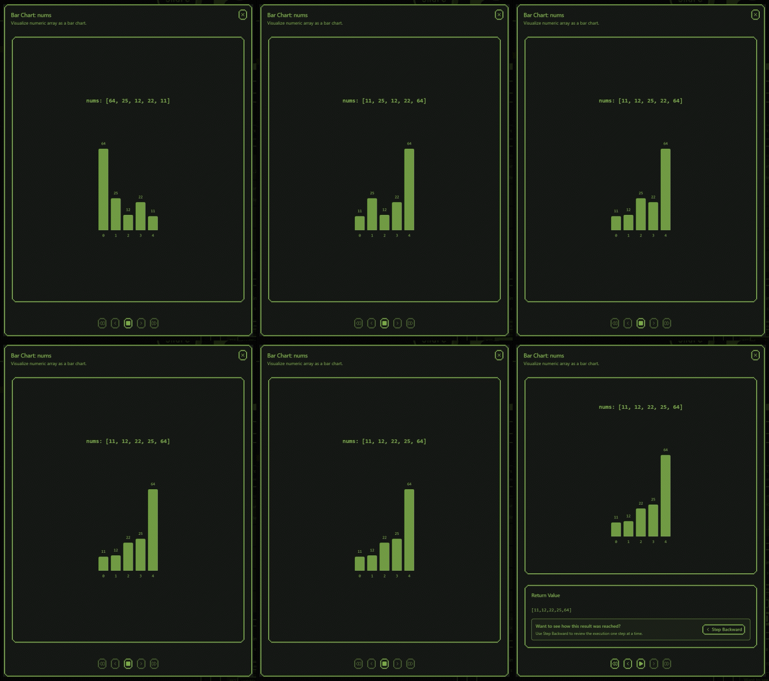
https://dsa-view-view.vercel.app/#s=j.eyJlIjoic2VsZWN0aW9uLcnQiLCJsIjoidHlwZXNjcmlwdCIsIm0iOiJ2ZXJpZmljYXRpb24iLCJ2IjoxfQ

When we visualize it, the basic pattern becomes obvious.

[5, 3, 4, 1, 2]
          ↑
       smallest

[1 | 3, 4, 5, 2]
              ↑
           smallest

[1, 2 | 4, 5, 3]

The algorithm is continuously growing a finished area from left to right.

That's Selection Sort.

Pick the smallest remaining value.

Put it next. And repeat. 🍥😸

---

🧠 What Did We Actually Learn?

Again, these three problems look completely different.

But each one introduces a useful way of thinking.

Trapping Rain Water

Use information from both sides to decide which part can already be solved safely.

Which side do I know enough about right now?

Top K Frequent Elements

Sometimes counting the data is only the first step.

Reorganize it into a structure where the answer becomes easy to retrieve.

Can I reorganize this information around what I actually need?

Selection Sort

Build the answer one permanent position at a time.

What value belongs in this position next?

So this time we saw

Two pointers
Frequency buckets
Selection

Three different mental models again.

And just like the previous problems, the difficult part is often not the syntax.

It's the changing state.

Which pointer moved?
What is the maximum now?
What is inside the Map?
Which bucket changed?
Where is minIndex?
Which part is already finished?

That's a lot to keep in our heads.

So instead, I want to view it. 👀👀

---

🎯 Conclusion

In this article, we looked at:

• Trapping Rain Water with two pointers
• Top K Frequent Elements with frequency buckets
• Selection Sort

And more importantly, we followed how their state changes while they run.

For Trapping Rain Water, we watched two pointers move inward while leftMax, rightMax, and water changed.

left →       ← right

For Top K Frequent Elements, we watched the same data change representation.

array
  ↓
frequency Map
  ↓
buckets
  ↓
result

For Selection Sort, we watched the sorted area grow one position at a time.

This is exactly the kind of thing I built DSA View View for.

https://dsa-view-view.vercel.app

You can write or load a TypeScript implementation, run it with your own inputs, and move backward and forward through the runtime.

If you are learning DSA too, try viewing one of these problems step by step.

And if there is a DSA problem you want me to cover next, please let me know in the comments!

I still have many algorithms to learn myself. 😸

Let's train our DSA muscles together! 💪

If you like DSA View View, please give it a star ⭐

https://github.com/nyaomaru/dsa-view-view

See you in the next article!